This post is about…

• a review of BEGAN:Boundary Equilibrium Generative Adversarial Networks

Greetings!

M: So, what episode was hot on Young jump this week?

G: Huh?

M: Young jump!

G: Dude, it’s golden week* ,man. There is no Young jump this week. Hello everyone, this is Guguchi.

M: What a Bummer… Hi, This is Maso!

*Golden week is a ‘literal’ cluster of 4 consecutive national holidays in the beginning of may. truly an Oasis for overworked Japanese.

BEGIN THE BEGAN!

M: Well, let’s begin the chat for today! Today’s topic is BEGAN. It was a buzzword on the geek world for … how long?

G: Ah, it came out on April, it’s been exciting people for a month. I think the heat
Well, How shall we describe BEGAN?

M: In short, you mean.

G: Yup.

M: Well, it is a method that aims to reduce Wasserstein distance between the reconstruction error of autoencoder for generated dataset and that of the autoencoder for real dataset…. at least that’s what people say.

G: Most importantly, it is a method that attempts to do away with min-max scheme. Its formulation is built to minimize a pair of objective function. The generated facial dataset is pretttty impressive.

M: This paper bewildered me at first. So many parts of the formulation confused the hell out of me.

G: Um, in fact, the Gaussian assumption of the reconstruction error took me off the guard, too. But why don’t we go over the notations first?

M: Sure thing! Let’s take a look at the equations in the paper. First… the reconstruction error for the autoencoder $D$ with parameter $\theta_D$ is given by

$$L(x; \theta_D) = \|x - D(x)\|_2$$

If $G$ is the generator, the goal is to make $L(x; \theta_D)$ approach 0 while keeping $L(G(z); \theta_D)$ and $L(x; \theta_D)$ as far apart as possible, in Wasserstein distance.

G: An then they insert something crazy here. They assume that these are all Gaussians. That is,

$$L(x; \theta_D) \sim \mathcal{N}(m_1 , C_1)$$ $$L(G(z) ; \theta_D) \sim \mathcal{N}(m_2 , C_2)$$

M: In fact, they say “We found experimentally, for the datasets we tried, the loss distribution is, in fact, approximately normal.” The Wasserstein distance between two Wasserstein distance is given by:

$$W(\mu_1, \mu_2) = \|m_1 - m_2 \|_2^2 + trace(C_1 + C_2 - 2C_2^{1/2} C_1 C_2^{1/2})^{1/2})$$

which in the case of dimension 1 is given by

$$W(\mu_1, \mu_2) = \|m_1 - m_2 \|_2^2 + (c_1 + c_2 - 2 \sqrt{c_1 c_2})$$

G: Then they make the somewhat mysterious assumption that

$$\frac{c_1 + c_2 - 2 \sqrt{c_1 c_2}}{\|m_1 - m_2 \|_2^2}$$

is constant, so that

$$W(\mu_1, \mu_2) \propto \|m_1 - m_2 \|_2^2$$

M: Maybe it is not TOO wierd, because all its saying is that the variance is proportional to mean square. umm. To me, the place that goes wierd on this paper is from 3.2, the GAN objective.

G: Well, let us first rephrase they explain this section. They claim that, there are two ways to maximize the Wasserstein distance above,

$$\begin{align} (a) \begin{cases} W(\mu_1,\mu_2) \propto m_1 - m_2 \\ m_1 \to \infty\\ m_2 \to 0\\ \end{cases} \\ (b) \begin{cases} W(\mu_1,\mu_2) \propto m_2 - m_1 \\ m_1 \to 0\\ m_2 \to \infty\\ \end{cases} \end{align}\$$

They select (b) for their purpose here because they want $L(X)$ to go to $0$. They achieve this by sequentially decreasing the two equations below:

$$\begin{align} \mathcal{L}_D &= \mathcal{L}(x;\theta_D) - \mathcal{L}(G(z;\theta_G);\theta_D)\\ \mathcal{L}_G &= \mathcal{L}(G(z;\theta_G);\theta_D)\\ \end{align}\ $$

M: There! Up until today (in the world of GAN), we increased W-distance by the discrimanator, and reduced the distance by the generator. The roles are inverted!!! Let us summarize what they are doing pictorially.

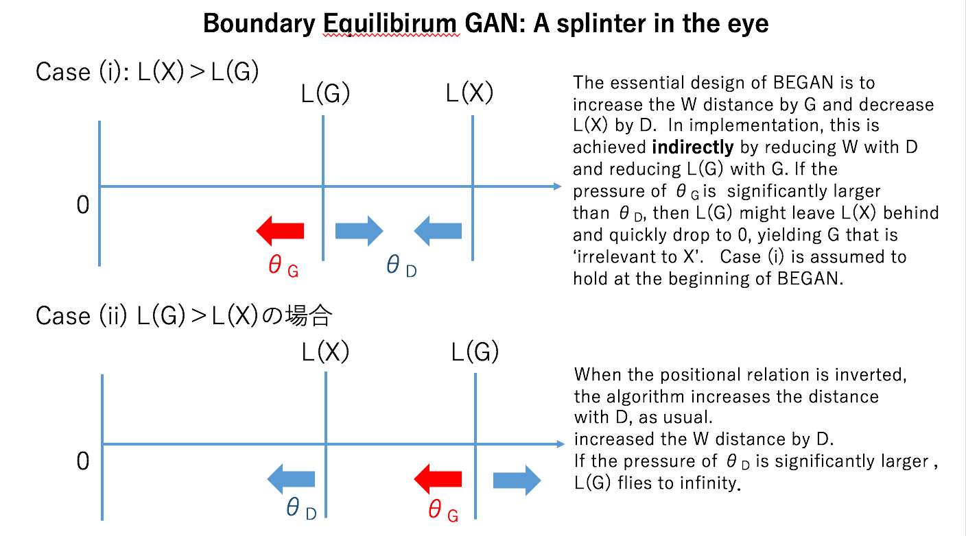
G: Well, it seems that your claim is not always the case when $L(X) < L(G)$. D increases the W distance, as usual.

M: Um, the paper makes the following claim:

In early training stages, G tends to generate easy-to-reconstruct data for the auto-encoder since generated data is close to 0 and the real data distribution has not been learned accurately yet. This yields to L(x) > L(G(z))

At least in the beginning, the Case (i) holds. What I am afraid of is that, in the formulation like this, L(G) might leave L(X) behind and quickly drop to 0 if we are not careful about the learning rate of $\theta_G$. And I really feel uncomfortable here. I feel we come back to max min vs min max issue that you mentioned in the previous episode.

The story of GAN, or at least the justification of GAN, was to produce G that can endure the worst D. In principle, its goal was to pull G into X. So, for this problem, I expect L(G) to be pulled into L(X) that approaches to 0 on its own. But all of sudden, as you look at this, the formulation, L(X) is drawn to 0 indirectly by L(G).

G: Well, in order to L(G) to not to drop too quickly, the gradient with respect to $\theta_G$ must be smaller than the gradient with respect to $\theta_D$. At some point, L(X) and L(G) will pass one another and we will reach the situation (ii) of L(G)> L(X). When this happens, if the gradient with respect to $\theta_G$ remains to be smaller than the gradient with respect to $\theta_D$, L(G) will fly off to infinity! So we must do something when this passover takes place.

M: I guess your concern, and my concern partially, are taken care of by equilibrium at 3.3.

$$\gamma = \frac{E[L(G)] }{E[L(X)]}$$

They use control theory to make sure that the ratio is kept constant at $\gamma$. umm.

G: You are talking about this equation.

$$\begin{align} \mathcal{L}_D &= L(x) - k_t \cdot L(G(z_D))\\ \mathcal{L}_G &= L(G(z_G))\\ k_{t+1} &= k_t + \lambda_k(\gamma L(x) - L(G(z_D)) \end{align}\ $$

M: Right, right! Let us put $e = \gamma L(x) - L(G(z_D)$. If e is too large, that is if L(G) is too small, we increase k so that L(X) will come along with L(G). If e is minus, or approaches 0 so that there will be instability in the ‘ratio’ they mentioned to be constant in the Wasserstein evaluation, we decrease k.

G: Well, looks like a formulation for which the pass-over DOES in fact takes place often. VERY often. Bad thing can happen, as far as what we see pictorially. I see many people implementing this algorithm, and they all seem to be having hard time getting the algorithm to work to its full potential. (musyoku , underfitting , rcalland）

M: Umm! it sounds interesting to checkout the trajectory of L(X) and L(G). We might be able to learn from the cases in which the algorithm does not work.

G: Give me GPU. GIVE. ME. GPU.

M: Give me Grants…